There are many questions on Metaculus about the behavior of asset prices on financial markets. Some of these questions can be quite difficult to answer using intuitive judgment. As an example, take this question (on which the community forecast may need some refreshing as of the time of publication of this notebook):

How would we go about forecasting this question with this definition of "correction"? One approach may be to look at past data for the S&P 500, possibly corrected for inflation in some way, and look at the base rate for corrections happening in the past. We can then use reference class forecasting to get a rough estimate of when the next correction should take place. In doing this we're throwing out all of the extra information we know about the index which might help us get a more precise estimate of the odds, but as a consequence we don't have to add additional sources of bias to our estimate by using some specific model or relying upon some specific story about how S&P 500 prices behave. This is an example of the classic bias-variance tradeoff in statistics.

In this notebook I'll try to talk about how we might take into account more information than simple base rates when making these kinds of forecasts. These inevitably involve having some kind of model of how asset prices work which might be wrong, but the possibility of adding this kind of bias is often compensated for by the lower variance you can expect.

## Martingales

The most naive model about asset prices which works especially well at high frequencies is that they are *martingales*. A [martingale](https://en.wikipedia.org/wiki/Martingale_(probability_theory) is a process whose expected future value at any point in time is always equal to its current value. In other words, you can neither make nor lose money on average by making trades on a market where the price is a martingale. The simplest martingale is a random walk: imagine that the asset price goes up by a fixed amount with a 50% chance and goes down by the same amount with a 50% chance in each time period. This exact model doesn't work well for asset prices, but thanks to the [central limit theorem](https://en.wikipedia.org/wiki/Central_limit_theorem) many martingales end up looking quite similar to each other when we zoom out, so you might be able to get some mileage out of even this seemingly very naive model. If we don't want to deal with these discrete time steps, the continuous version of a random walk exists and is called [Brownian motion](https://en.wikipedia.org/wiki/Brownian_motion).

The most serious problem which will immediately jump out at anyone who has looked at a S&P 500 chart is that the S&P 500 is most definitely not a martingale: it has a strong tendency to go up by around 8% a year in real terms over long time horizons. To account for this, we need to combine the random walk with an upward moving trend, preferably an exponential trend to reproduce this 8% per year growth that we observe empirically.

Suppose that we try to make this formal in a way that a computer will be able to simulate it. Suppose the S&P 500 stock price at time t is S(t). In a small time window \Delta t we want the stock price to change by a fixed amount \mu S(t) \Delta t, perhaps with \mu \approx 8 \%/\textrm{year}, to reproduce the empirical long-run growth rate of the stock market. On top of this we want to add some randomness with some scale factor \sigma, and we can represent this by a normal distribution \sigma S(t) \sqrt{\Delta t} N(0, 1) where N(0, 1) is a standard normal random variable, with mean 0 and variance 1. We end up with a "law of motion"

\Delta S(t) = S(t + \Delta t) - S(t) = \mu S(t) \Delta t + \sigma S(t) \sqrt{\Delta t} N(0, 1) 

This is something we can simulate by simply choosing three parameters \mu, \sigma, \Delta t. \mu and \sigma we can estimate empirically, and they turn out to be about \mu \approx 8 \%/\textrm{year} and \sigma \approx 20 \%/\sqrt{\textrm{year}}. Our choice of \Delta t depends on the scale at which we want to do forecasting, but overall we should choose it to be much smaller than 1/\mu and 1/\sigma^2. For the S&P 500, a choice of \Delta t = 1 \, \textrm{day} would be suitable for most medium term forecasts.

If we want to work in continuous time, we can also use stochastic calculus to get rid of this sampling period \Delta t entirely. In the language of stochastic calculus the equation we just wrote would be a *stochastic differential equation* and it would read dS/S = \mu \, dt + \sigma \, dz. Those familiar with ordinary calculus can probably understand the motivation to want to work with differential equations instead of discrete difference equations: we can often get tractable analytic and closed-form solutions to differential equations which we might not be able to do for difference equations. This is also true here: the process we just wrote down would be classified as a geometric Brownian motion with drift, and its behavior is very well understood thanks for various theorems in stochastic calculus.

Now we have a strategy for forecasting the question I originally quoted in the first section. Here is how we would do it: we take the discrete law of motion above with the mentioned parameter settings and simulate lots of sample paths out from it, maybe around 1000, in a Monte Carlo fashion. For each sample path we record the date of the first correction, and then we put those in a list and plot a histogram to see what the distribution looks like. We can then base a forecast on the Metaculus question on this distribution.

## Weaknesses

Whenever we specify an explicit model for an asset price, we'll be simplifying what's actually going on. This adds a source of bias to our forecasts, but we hope that the lower variance obtained compared to base rate forecasting makes the tradeoff worth it. Nevertheless, insofar as we can do it at low cost, we should try to eliminate these sources of bias.

In fact the geometric Brownian motion model of stock prices fails on many different levels. Both the expected return \mu and the volatility \sigma on the stock market vary over time. Here is a plot of the VIX, which is a market-based estimate of S&P 500 volatility (it's really the square root of an estimate of variance, but this difference doesn't matter much here):

![](https://metaculus-media.s3.amazonaws.com/user_uploaded/0b40b638db5b9d925f2b8f1f1ab9c5f8.jpeg)

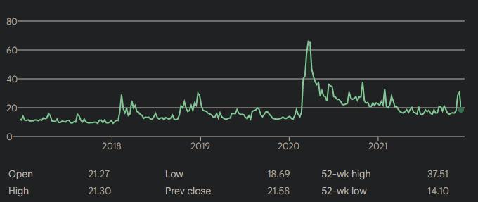
*Does that look constant to you?*

  


This can be even more dangerous when we're forecasting tail events because their odds tends to be highly convex in the parameters of the model; in other words, we'll be dramatically underestimating their chances of occurring if we simply let \mu, \sigma equal the *average* return and the *average* volatility on the stock market respectively. For example, 20 \% per year of volatility is equivalent to about 1 \% a day, so if we believe our model and assume daily S&P 500 movements follow a normal distribution, we should predict that 10 \% daily price moves in the S&P 500 are 10 \sigma events, which for a normal distribution have odds of 7.6 \times 10^{-24}. In other words, we would expect to see one such event roughly every 1.3 \times 10^{23} days, which is a number of orders of magnitude above the age of the universe. However, Wikipedia [helpfully lists](https://en.wikipedia.org/wiki/List_of_largest_daily_changes_in_the_S%26P_500_Index) the biggest daily price moves in the history of the S&P 500 index, and we can see that there have been 10 moves bigger than 10% in either direction since 1923. 

The problem is that *extreme price moves are convex in volatility*. During the peak of COVID-related volatility in markets in March 2020, the VIX index was higher than 80 on some days, corresponding to an annualized volatility of over 80 \%. That's approximately 4 \% daily volatility, and with that level of volatility we'd expect to see a 10 \% price move every 160 days or so. Even this is going to be an understatement since there is always the chance that volatility can rise even higher, and in these extreme regimes even at fixed volatility daily stock price movements might fail to follow a normal distribution.

However, even though the geometric Brownian motion model fails catastrophically in forecasting these kinds of tail events, it's actually quite good for forecasting "middle of the distribution" events such as the date of the next S&P 500 correction. The lesson here is that you should understand the success and failure modes of the models you have at your disposal, and if the explicit models you have are no good, you'll want to either build a new model which is good or just stick to reference class forecasting. As an exercise, you might think about how you would forecast on the following question:

We can improve the geometric Brownian motion by also making volatility itself a stochastic process to add this convexity into the model or by bootstrapping returns from past price data, but for the purposes of this notebook I'll stick to this simple model and move onto how else we might use it to do forecasting without actually needing to rely on Monte Carlo simulations.

## Technical primer on options

For an asset price forecaster, option price data is invaluable information. An [option](https://en.wikipedia.org/wiki/Option_(finance)) is an instrument that you can own which gives you the right, but not the obligation, to buy or sell an underlying asset at a predetermined *strike price* either until (American style) or at (European style) an *expiration date*. If the option grants its owner the right to buy a stock it's called a call option, and if it grants the owner the right to sell a stock it's called a put option.

We can see why they are so important to forecasters by looking at the payoff function of an option at expiration. Suppose that we're dealing with a call option and the price of the underlying stock at time t is S(t), the expiration date of the option is T and its strike price is K, and for simplicity assume the option is European style so we can only exercise it at expiration. Then if it happens that S(T) \leq K the option would expire as worthless since it would give us the right to buy a stock at a price K whose market price is actually below K, while if it happens that S(T) > K we can exercise the option to buy the stock at K and then sell it on the market for S(T), thus profiting by the difference S(T) - K. In short, our payoff from the option is equal to \max \{ 0, S(T) - K \}.

This particular function will be familiar to those who know about neural networks: this is simply the activation function of a [rectifier](https://en.wikipedia.org/wiki/Rectifier_(neural_networks)). It's useful in machine learning because it provides a relatively inexpensive way to add nonlinear activations to a neural network, and its role in finance is actually similar. Thanks to some approximation theorems we can actually infer what the price of a hypothetical asset whose payoff is defined by an arbitrary continuous function f(S(T)) would be just by approximating f using some linear combination of option positions.

In practice it's also useful to know about the [Black-Scholes model](https://en.wikipedia.org/wiki/Black%E2%80%93Scholes_model) of option pricing to interpret option price quotes, since often they will quote a quantity called "implied volatility" as a way to standardize the price quotes of many different kinds of options at different strike prices, expiration dates, *et cetera*. It's not difficult to explain the basic idea behind the model. Suppose that we have an underlying asset S following the geometric Brownian motion with drift we described earlier, dS/S = \mu \, dt + \sigma \, dz. We want to define the "implied volatility" of an option as the \sigma such that the option would have the price we empirically observe given its strike and time to expiration. In other words, we take the price of the option and its parameters, and we solve for the \sigma that would make all of that consistent.

To do this, we actually need to figure out how to calculate the "right" price for an option in this geometric Brownian motion setting. A naive approach to price an option on this asset might be to just do what's called "risk-neutral pricing": for an option that expires at time T and has strike price K we simply solve the differential equation forward to compute the probability distribution of S(T), then we use it to compute the expected value of \max \{0, S(T) - K \} by integration, and what we end up with is the price of our option.

This idea almost works, but there are two problems with it. One is that we really ought to discount a payoff in the future by some interest rate, since money we get in the future will be worth less than money we get today. Two is a bigger problem. S itself is not a martingale in this setup, so if we have two times t\_1 < t\_2 then it's not true that S(t\_1) is the expected value of S(t\_2) conditional on what we know at time t\_1, so there's no particular reason to expect our integral to equal the price of an option on S either. The problem is that S is a risky asset and so has a risk premium, and we really ought to adjust for that somehow in our calculation.

To overcome these issues we would like to price the option by arbitrage, that is, we would like to write down an explicit strategy to make money if the price of the option disagrees with the price that our model predicts for it. Since the only assets available to us are the option and the underlying asset, this strategy must consist of holding these at some weights relative to each other.

Here is a portfolio that works: suppose the price of the option is V(S, K, T ) where S is the current price of the underlying, K is the strike price and T is the time until expiration. The portfolio that's long 1 unit of V and short \partial V/\partial S units of S at every time is called the *delta portfolio*, and it turns out to be the key to the arbitrage argument. To see this, notice that the instantaneous return on this portfolio is equal, by [Ito's lemma](https://en.wikipedia.org/wiki/It%C3%B4%27s_lemma), to

dV - \frac{\partial V}{\partial S} dS = \frac{\partial V}{\partial S} dS + \frac{1}{2} \frac{\partial^2 V}{\partial S^2} (dS)^2 - \frac{\partial V}{\partial T} dt - \frac{\partial V}{\partial S} dS = \frac{\sigma^2 S^2}{2} \frac{\partial^2 V}{\partial S^2} dt - \frac{\partial V}{\partial T} dt 

The key here is that the stochastic "random walk" part of dS cancels out because we chose the weights of V and S carefully, so *the delta portfolio is risk-free*. That means that if the risk-free rate of return is r, we can assume by arbitrage that the return on the delta portfolio is also r, which leads to the equation

\frac{\sigma^2 S^2}{2} \frac{\partial^2 V}{\partial S^2} - \frac{\partial V}{\partial T} = rV - rS \frac{\partial V}{\partial S} 

This is the famous Black-Scholes equation. To specialize it to the case of a put option or call option, we solve it with the boundary condition that the payoff when there's no time until expiration is just equal to the payoff of the option itself: V(S, K, 0) = \max \{ 0, S - K \} for a call option, for example. 

What's important about the Black-Scholes equation is not the specific equation itself but that we can actually price options by arbitrage, since it's not difficult to prove that solutions to this differential equation exist and are unique given the boundary condition at T = 0and a few other boundary conditions to ensure that the solution is sensible. Importantly, the mean return \mu does not show up in the equation at all, which means that option prices are independent of \mu given the current underlying price S. This is a deep point: option prices can't tell us about expected returns! When we want to do forecasting, therefore, we have to obtain some idea of what we can expect \mu to be in some other fashion, since it's impossible to extract it from option prices.

In the special case that r = 0 (which is quite relevant nowadays) and \mu = 0 (which we can assume without loss of generality since V doesn't depend on \mu) the Black-Scholes equation is equivalent to V being a martingale. In this special case, the price of the option is indeed the expected value of its future payoff. This means we can actually find V explicitly in the case r = 0 by computing the integral that I mentioned earlier, just with taking care to set \mu = 0 to get rid of the risk premia issues.

Our discussion here was implicitly assuming V is an European option, but what if it's an American option? It turns out that under certain conditions European and American options are equivalent, because it's never optimal to exercise an American option before expiration (rather than selling it), but since this equivalence doesn't always hold I'll refrain from saying more about it here and stick to European options.

## Forecasting using option prices

Let's do a concrete example. Take this question:

It turns out we have enough information at our disposal to forecast this without relying on any kind of Monte Carlo simulations, purely relying on option price data. I'll explain what I did to forecast this question step by step.

First, I went on [Deribit](https://legacy.deribit.com/main#/options?tab=BTC-30SEP22) and looked at the prices of the options with the longest time to expiration, which in this case is about 3 months before December 31 2022. The "IV" columns denote the implied volatility calculated using the Black-Scholes model with r = 0 for each of the strikes in the list. They won't be all equal because of the convexity problem I discussed earlier: a typical situation is that the implied volatility of options with strike prices further away from the current market price of the asset will be higher. However, in this case the implied volatilities are all within a relatively narrow band of from 90% to 100% annualized, so in the price range we're talking about the market is signaling that deviations from normality in returns are not too significant.

Now, let's assume for the moment that \mu = 0 and figure out what we should forecast in this case. dS/S = \sigma dz means that d \log(S) = \sigma dz - \frac{\sigma^2}{2} dt, so the distribution of the logarithm of the BTC price in about one year should be roughly the current forward price plus N(-\sigma^2/2, \sigma^2) with the two entries corresponding to mean and variance respectively. We can check that the forward for this date is roughly 53300 dollars, and we can add a further 1000-2000 to that because the forward prices seem to be trending up over time and we don't have actual data for 31 December 2022. If we assume \sigma = 100 \% annualized for simplicity, we end up with a distribution

\log(\textrm{price}) \sim N(\log(55000) - 0.5, 1) = N(10.4, 1) 

A rule of thumb is that the 25-50-75th percentiles of a normal distribution N(\mu, \sigma^2) are given by \mu - 0.674 \sigma, \mu, \mu + 0.674 \sigma. In this case this gives us 16747 - 32859 - 64472 for the three percentiles.

Why is the median so much lower than the current spot price? This is because the distribution of the future price is lognormal with a high variance, and in this case the *average* value of a lognormal is much higher than its *median* value. In this case the average value of our forecast is actually exactly the current forward price, but because of the skew of the lognormal distribution the median ends up being quite a bit smaller.

Now, we can add some mean return on top of this calculation easily by shifting these percentiles up or down by whatever we think is a reasonable estimate of the expected return on BTC. I think something much higher than 10 \%/\textrm{year} for this is hard to justify, but since we can't actually infer this from the option prices you have to make up your own mind about what you think is a reasonable estimate there.

I'll end this section with another question about the future volatility of BTC. This one we don't have any reliable option price data for, so you'll have to use your own judgment to forecast on it, but given what we learn from this kind of question we can leverage the information using the methods discussed in this notebook to forecast on all kinds of other questions about the BTC price process.

## Conclusion

Overall, the methods I've discussed in this notebook work well when we're forecasting events that are not too extreme and that we either have good historical data or good current market prices to base our forecasts on. While the tools themselves are good, be careful not to use them beyond the domain where they give good performance!